Overview

In this project, we focus on shooting our own images and finding correspondences in between them to a lot of interesting things. First, we warp images and calculate its rectification, which allows us to see images as if they were posted in front of us, rather than in perspective. Second, we can use this information to blend images together and form panoramic views. We continued this in 4B, when we attempted to automate how we got our correspondence points and filtered them to get just the right amount in the right places.

Shoot the Pictures & Recovering Homographies

Here are some pictures from the rooftop of an apartment. A homography is a 3x3 matrix which represents a transformation between a pair of images. We can recover a homography by using pairs of corresponding points. The points on the pictures above represent the corresponding points. To implement this function, I went through each pair of points and created a system of equations to obtain the homography matrix’s coefficients, of which there will be 9 values. I then solved it with a least squares solver and reshaped it into a 3x3 matrix.

Rooftop

Forest

Bush and Water

Warp the Images & Image Rectification

For this we use a function that takes in an image and a homography matrix. I define the image’s corners in the same order I took the points in for image rectification. I then warped those corners with the input homography matrix and calculated a bounding box for my resulting image. Then, I found all the values within the bounding box and applied the inverse homography matrix to them. Finally, I ran interpolation with griddata to achieve the final result. To get the images for rectification, I found images with rectangles and chose its destination coordinates to be an arbitrary value found in the caption of the images below. My image took very high resolution images that the code couldn’t process, so I resized my images, resulting in a little blurriness. This is reflected in the rectified images as well.

Original Painting

Rectified Painting

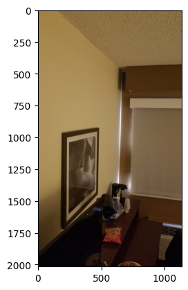
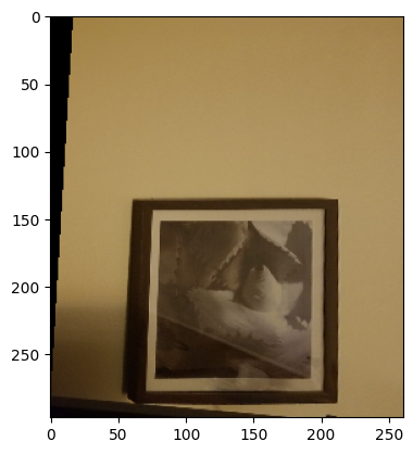
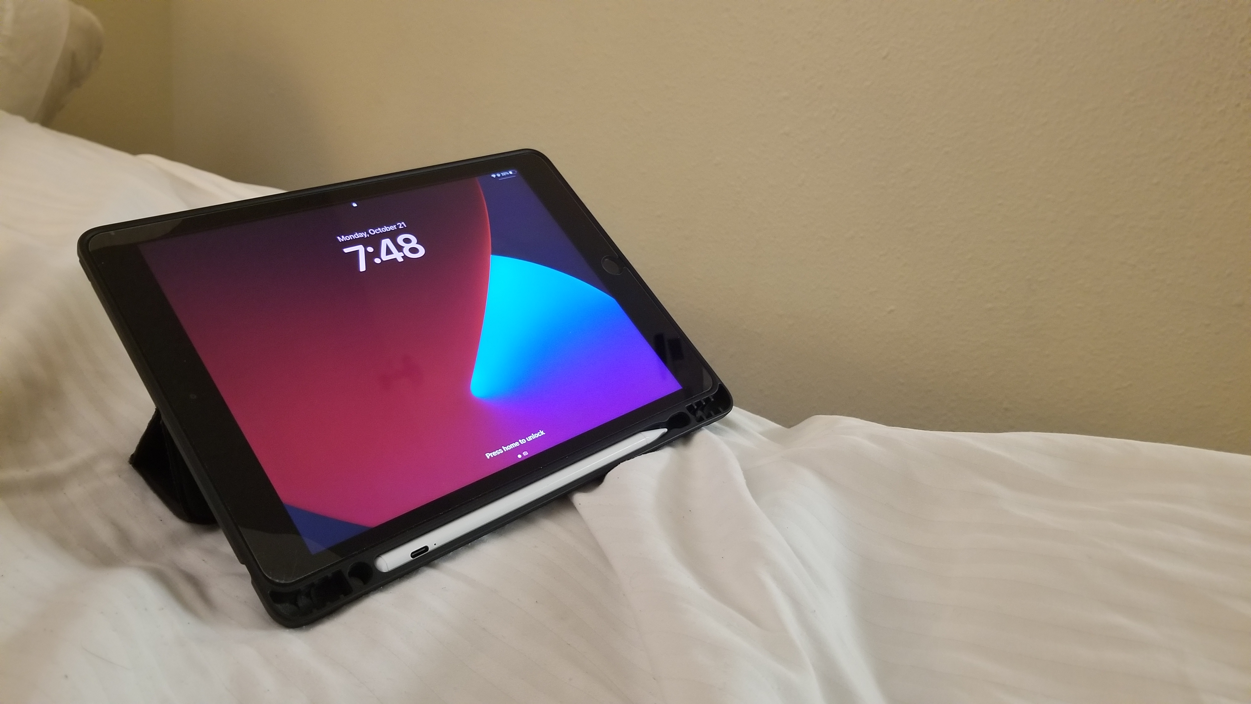
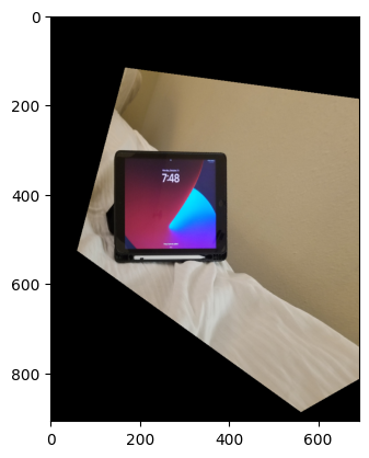
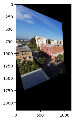
Original iPad

Rectified iPad

Blending Images

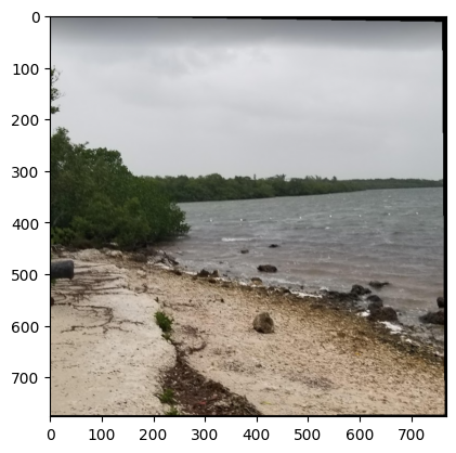
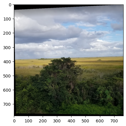
To blend images, I used some of my code from Project 2 as reference, particularly the part regarding blending with Laplacian pyramids. The key difference in this section is computing the mask that allows us to blend both images. Previously, it was a half white, half black mask because we wanted half of an apple and half of an orange. This time, we need to compute a distance map that determines how much of an impact the images should have in the blend for different parts of the total image. We also need to create a canvas that can hold both images, so we have a true merging of images, instead of one just overlapping the other.

Result 1

Result 2

Result 3

Project 4B: Feature Matching & Autostitching

Harris Corner Detection

We are given a function for this section that is able to detect Harris response values within an image, primarily using the corner_harris function from skimage.feature. Harris corners near the edge are discarded. Then, we essentially find the maxima across these values to identify the corner points. Importantly, we must input a grayscale image.

Naiive Harris Corner Detection

Adaptive Non-Maximal Suppression

To implement Adaptive Non-Maximal Suppression, we want to select a specific set of strong corners by applying a robust condition to filter and find those points. We find other corners within the image with stronger Harris value and keep track of the smallest distances to these stronger corners. Then, we can get however many of the strongest corners we’d like, leading to a more evenly distributed set of points as shown below.

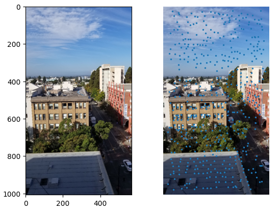ANMS Result

Feature Descriptor Extraction + Matching

Here, for every corner we found in Adaptive Non-Maximal Suppression, we see if a 40x40 window around the points fits within the image. If it does, downsample it and look at every 8x8 patch. Then, we normalize each of these patches and return a list of all these descriptors. We run this algorithm on both images to get two descriptor sets. Then, for feature descriptor matching, we look at the first image’s descriptor set and find the indices of the two nearest neighbors in the other image’s descriptor set. Next, we apply Lowe’s ratio test, which finds matches where the distance to the closest neighbor is significantly smaller. For all places where this condition is satisfied, we add its pair of indices.

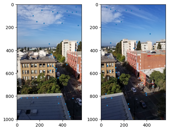Matching Points between both images

RANSAC

To implement 4-point RANSAC, we use steps outlined in lecture. In summary, we select four feature points at random, compute the homography, computer inliers that meet a specific distance condition, keep the largest set of inliers, and finally re-compute the least-squares H estimate on all the inliers. For each iteration, select 4 random correspondence points from the previous section and compute its homography. We use that H value to project the first image’s points onto the second image’s points. We calculate the distances between the projected and actual points for the second image and see which values are beneath the threshold. If the inlier count at this point of the iteration is more than we found previously, we update that counter and recalculate the resulting homography, which ultimately gets returned after all the iterations.