Overview
In this project, our goal is to implement and deploy diffusion models. Part A focuses on adding noise and denoising images through various techniques. It also looks at how certain prompt embeddings lead to unique images, as we play around with inpainting and making hybrid images. Part B is more advanced. The goal here is to train our own models on the MNIST dataset. There are different UNet architectures being used, leading to different training loss graphs and results.Part A: The Power of Diffusion Models!
Setup
Here are some pictures from the rooftop of an apartment. A homography is a 3x3 matrix which represents a transformation between a pair of images. We can recover a homography by using pairs of corresponding points. The points on the pictures above represent the corresponding points. To implement this function, I went through each pair of points and created a system of equations to obtain the homography matrix’s coefficients, of which there will be 9 values. I then solved it with a least squares solver and reshaped it into a 3x3 matrix.|
|
Part 1.1: Implementing the Forward Process
In this part, we aim to take a clean image and produce a noisy image by sampling from a Gaussian. To accomplish this, I first get the alpha bar by getting the correct alpha_cumprod value at its respective timestep. Then, I calculate a random epsilon value and use all this info in equation 2 to get the noisy image.|
|
|
Part 1.2: Classical Denoising
Now, we use Gaussian blur filtering to try to remove the noise with a kernel size of 5 and sigma of 1. This is primarily accomplished using torchvision.transforms.functional.gaussian_blur.|
|
Part 1.3: One Step Denoising
We use a pre-trained diffusion model to denoise, which is a UNet that’s been trained on a very large dataset. Using the UNet, we first estimate the noise in the noisy image. Then, we use the formula in equation 2 (as shown in 1.1) to create the clean image given the noisy image, using the noise estimate in the place of epsilon. This gives us a blurry image without the noise seen in 1.1, as well as providing a better output than 1.2.|
|
Part 1.4: Iterative Denoising
In this part, instead of one-step denoising, we plan to denoise iteratively. We create a list of timesteps from 990 to 0, with intervals of 30. So at each denoising step, we use formula 3 to reduce the noise within the current iteration of the image. This is accomplished by calculating the alpha and beta values at the current and incoming timestep and running unet to get the noise estimate of the current image.|
|
|
|
|
|
|
|
Part 1.
Part 1.5: Diffusion Model Sampling
I use torch.randn to make noise and then call the iterative_denoise from the last part to generate the image.

5 Sampled Images
Part 1.6: Classifier Free Guidance
To use this technique, we use a lot of code written for iterative denoising. The difference is we have conditional and unconditional prompt embeddings. The unconditional prompt embedding is just null and we calculate the Unet for both these values instead of just one before. Then, we pull the noise estimates for both the Unets and use the formula below with the pre-specified scaling factor. The rest is the same.

5 Sampled Images
Part 1.7: Image-to-image Translation
In this section, we add noise to an image and try to bring it back without any conditioning. The goal is to get back an image very close to the test image. Once again, we try this with a variety of noise levels.

Test Image

Doe Library

Blackwell Hall
Part 1.7.1: Editing Hand-Drawn and Web Images
Similar to the last part, we use the same prompt embeddings and iteratively denoise with cfg. However, now I’ve downloaded an image of Mike Wazowski and ran the forward method on it. We then run the method with varying i_start noise levels, ultimately showing that progression of images that leads to a Wazowski by the time it is 20. At the beginning with lower noise levels, there’s drastically different images.

Mike from Monsters, Inc.

Hand-Drawn House

Hand-Drawn Face
Part 1.7.2: Inpainting
In this section, we have an image and a binary mask. The goal is to keep the image intact where the mask doesn’t exist and input a new image into the mask. In the example below, we have the Campanile whose top is masked and a new image has to be processed. We use a lot of logic from the iteratively denoised cfg method with some modifications at the end. We take the result of each iteration and then run the formula below with the original image. This becomes the new image we work on every iteration of the loop.

Campanile

Mike image + mask

Inpainted result for Mike

Blackwell Hall img + mask

Inpainted result for Blackwell Hall
Part 1.7.3: Text-Conditional Image-to-image Translation
The logic of this section is essentially the same as 1.7.2, but instead we guide the projection with a text prompt by changing the prompt embedding. As you can see below, the image becomes more like what it should as the noise level increases.

Campanile

Blackwell Hall

Salesforce Tower
Part 1.8: Visual Anagrams
This was the coolest section to implement because we’re creating an optical illusion. At one orientation, the image looks like something, and then when it is flipped, it’s something entirely different. Once again, we use the logic behind iteratively denoising with cfg. Since we are creating two images in one, we need two conditional and unconditional prompt embeddings each. We use a pair containing one each to run the Unet twice and calculate that specific noise estimate, and then do it again on the second pair. When calculating these, we use the below formula. Most importantly, we must flip the image for the second Unet and then flip the outputs back. Once we have our two noise estimates, we calculate cfg noise estimate of each and then average those. That will be the noisy estimate for the image calculation.
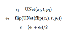
Part 1.8's Algorithm
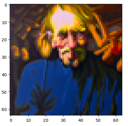
"an oil painting of an old man"
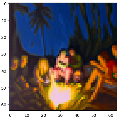
"an oil painting of people around a campfire"
"a lithograph of a skull"
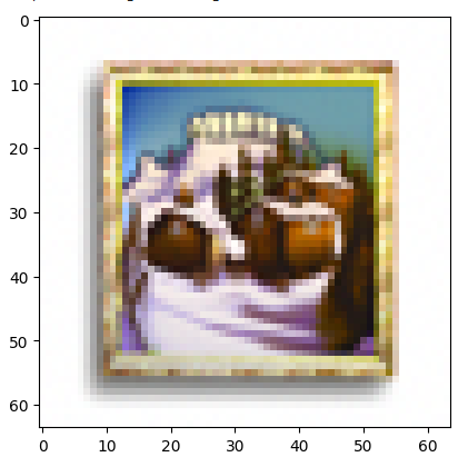
"an oil painting of a snowy mountain village"
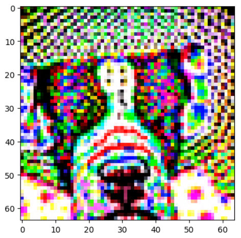
"a photo of a dog"
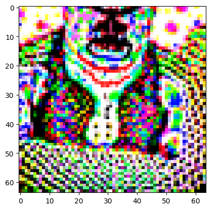
"a photo of a hipster barista"
Part 1.9: Hybrid Anagrams
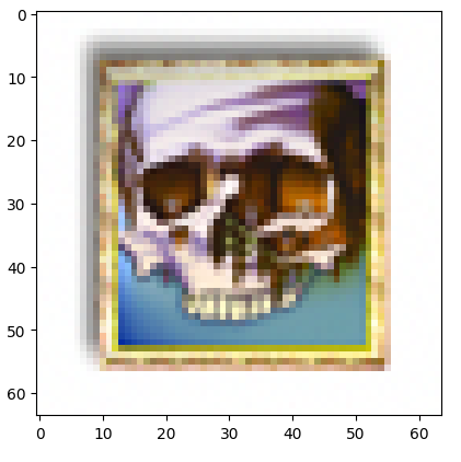
In this section, our goal is to trick the viewer into seeing a certain image up close and a different image further away. Once again, we use the cfg noise estimate from two pairs of conditional and unconditional prompt embeddings. To pull off this trick, for the image we want to see up close, we use a low pass filter and then for the one we want to see further away, we use a high pass filter. We combine these filters to get a new noise estimate and then continue our code. The formula is also below for reference.
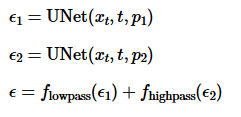
Part 1.9's Algorithm

"a lithograph of a skull" and "a lithograph of waterfalls"

"a rocket ship" and "a pencil"

"a lithograph of a skull" and "a photo of a dog"
Part B: Diffusion Models from Scratch!
Part 1: Training a Single-Step Denoising UNet
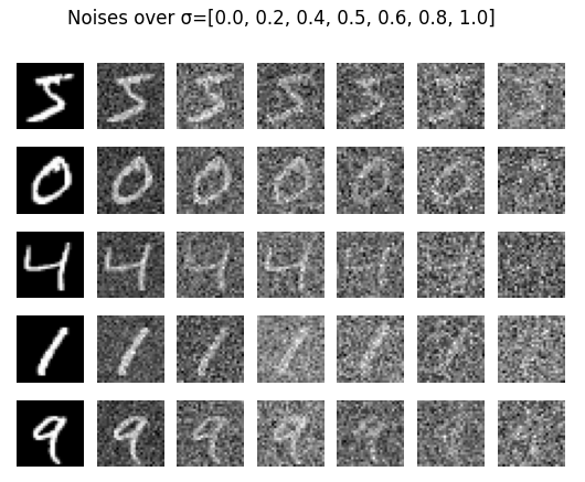
In this part, our goal is to train a denoiser such that we can take in a noisy image and obtain a clean image by optimizing the L2 Loss. The Unet architecture has a lot of operations that we needed to implement such as ConvBlock and UpBlock. These operations had to be put in a specific order with the appropriate number of input and output channels. Once that was completed, we ran 5 epochs to train the model and all the results are below.
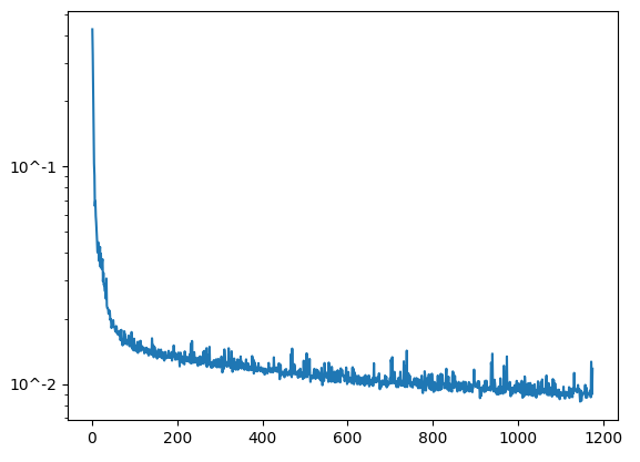
Training Loss Curve Plot
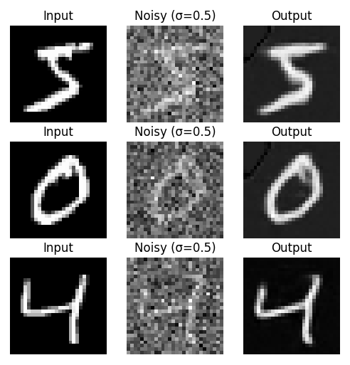
Results after epoch 0
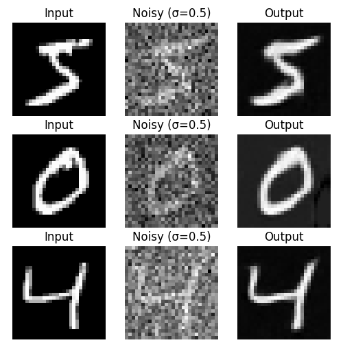
Results after epoch 5
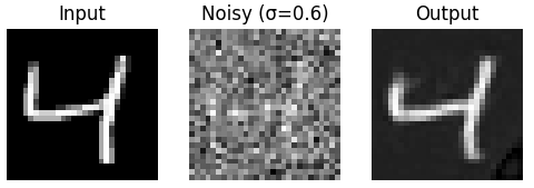
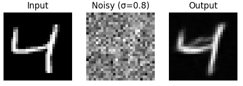
Below is the test digit on varying levels of noises. The last one is for when it is at 1.0, the screenshot was cut off.
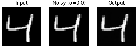
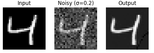
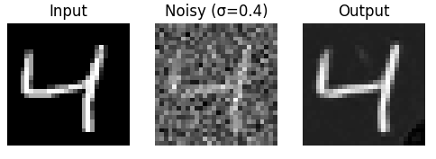
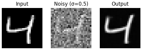

Part 2: Training a Diffusion Model
First, we add time conditioning to the Unet, which involves adding two FCBlocks based on t. We then add these results to the appropriate block based on the image from the spec. At this point, when we sample, we only include the unconditional value for epsilon. In part 2.4, we add class-conditioning to the Unet, which requires adding two more FCBlocks that use the c paramter. Essentially we want a 10% dropout rate, where c gets set to zeros. We multiply the result of the FCBlock before adding the time conditioning result from the last part.
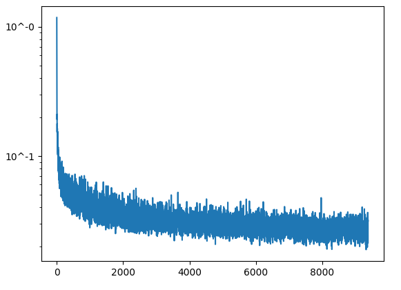
Training Loss Curve Plot
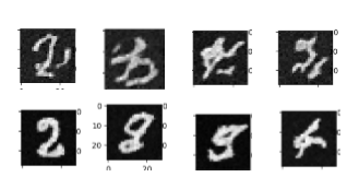
Results after epoch 0 (top) & epoch 5 (bottom)
After implementing class conditioning results below.
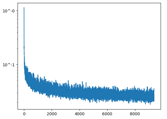
Training Loss Curve Plot
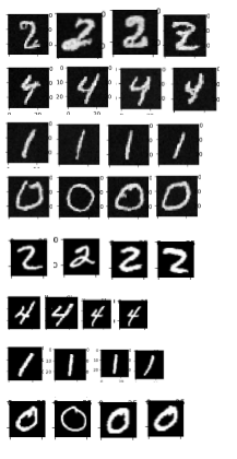
Results after epoch 0 (top 4 rows) & epoch 5 (bottom 4 rows)
|
|
|
|
|
|
|
|
|
|
|
|
|
|
|
|
|
|
|
|
|
|
Part 1.7.3: Text-Conditional Image-to-image Translation
The logic of this section is essentially the same as 1.7.2, but instead we guide the projection with a text prompt by changing the prompt embedding. As you can see below, the image becomes more like what it should as the noise level increases.|
|
|
|
|
Part 1.8: Visual Anagrams
This was the coolest section to implement because we’re creating an optical illusion. At one orientation, the image looks like something, and then when it is flipped, it’s something entirely different. Once again, we use the logic behind iteratively denoising with cfg. Since we are creating two images in one, we need two conditional and unconditional prompt embeddings each. We use a pair containing one each to run the Unet twice and calculate that specific noise estimate, and then do it again on the second pair. When calculating these, we use the below formula. Most importantly, we must flip the image for the second Unet and then flip the outputs back. Once we have our two noise estimates, we calculate cfg noise estimate of each and then average those. That will be the noisy estimate for the image calculation.|
|
|
|
|
|
|
|
|
|
|
Part 1.9: Hybrid Anagrams
In this section, our goal is to trick the viewer into seeing a certain image up close and a different image further away. Once again, we use the cfg noise estimate from two pairs of conditional and unconditional prompt embeddings. To pull off this trick, for the image we want to see up close, we use a low pass filter and then for the one we want to see further away, we use a high pass filter. We combine these filters to get a new noise estimate and then continue our code. The formula is also below for reference.|
|
|
|
|
|
Part B: Diffusion Models from Scratch!
Part 1: Training a Single-Step Denoising UNet
In this part, our goal is to train a denoiser such that we can take in a noisy image and obtain a clean image by optimizing the L2 Loss. The Unet architecture has a lot of operations that we needed to implement such as ConvBlock and UpBlock. These operations had to be put in a specific order with the appropriate number of input and output channels. Once that was completed, we ran 5 epochs to train the model and all the results are below.|
|
|
|
|
|
Below is the test digit on varying levels of noises. The last one is for when it is at 1.0, the screenshot was cut off.
|
|
|
|
|
|
|
|
|
|
|
Part 2: Training a Diffusion Model
First, we add time conditioning to the Unet, which involves adding two FCBlocks based on t. We then add these results to the appropriate block based on the image from the spec. At this point, when we sample, we only include the unconditional value for epsilon. In part 2.4, we add class-conditioning to the Unet, which requires adding two more FCBlocks that use the c paramter. Essentially we want a 10% dropout rate, where c gets set to zeros. We multiply the result of the FCBlock before adding the time conditioning result from the last part.|
|
|
|
|
|
|
|